Direction of Research
Summary Equations
As our thesis is concerned almost exclusively with the conical hopper, we shall mainly be using the three equations derived for the conical section in our future research.
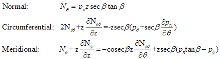
Because this is very new territory for us, and because it is initially imprudent to introduce too much complexity, for now, the above equations will be considered only for the axisymmetric loading conditions. This allows their simplification to the following (notice the lack of shear stress resultants):
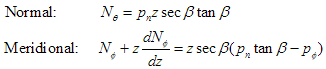
The meridional equation is actually a first order ordinary differential equation (ODE) which can be solved for a number of load cases of the distributed internal pressures, pn.
Sample load case 1 top Δ
Internal pressure is constant over the whole height of the hopper: pn = po.
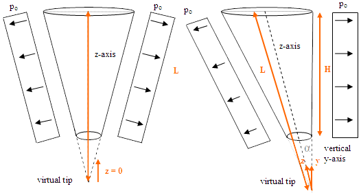
Fig. 11
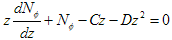
The ODE for the meridional stresses is in the form:
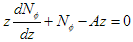
where A is a constant. The solution to this equation is:
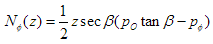
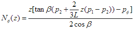
Its derivation is available in pdf format. This is the solution for the meridional stresses along the entire height of the hopper, with z = y = 0 at the bottom of the extended virtual tip. Notice that it is very easy to expand the above equation to an eccentric hopper, where z is no longer the vertical axis, simply by dividing by cosα, where α is the angle between the hopper axis and the vertical. Thus, for an eccentric hopper with constant internal pressure only, the above equations become:
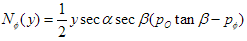
and
Sample load case 2 top Δ
Internal pressure varies linearly along the entire axis (z) of the hopper (hydrostatic pressure): pn = p1 + (p2 p1)(L-z)/L.
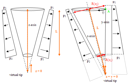
Fig. 12
This is a more complex case for the eccentric hopper, and the above diagrams bear witness to this. Because the position along the shell is described using the polar coordinate system (radius to z-axis and angle around z-axis), it is unnecessarily difficult to transform the system to the vertical y-axis, as this actually cannot be done with ease without reverting to a Cartesian coordinate system. This is because, in the y-axis, the radius, and hence the point of equal pressure around the shell, varies with θ (the circumferential angle), and lies in a plane perpendicular (going through the page) to the plane of all of the above parameters. The equations will, therefore, stay polar and defined in terms of the z-axis.
In the above system, the internal normal pressures are linearly distributed along the z-axis and the radius is taken to be perpendicular to this axis. This implies that, for example, assuming the right side is vertical, the pressure py at the top of the hopper on the vertical y-axis, but the point along the left side which is at the same pressure py does not have the same y value, but it does have the same z value. Conversely, the point at the top of the left side is at a much smaller pressure than p1. The right side never actually reaches this pressure because the hopper does not physically reach up to the equivalent point on this side.
The cone can be extended below the outlet to a virtual tip, as can the pressure distribution, and the z = 0 boundary condition needs to be situated at this virtual tip of the oblique cone. Note that L is the total length of the hopper from the virtual tip (z = 0) to the hopper-silo transition point. The relevant pressures along this length can be found from the desired distance along the hopper axis, and the required radii are given by: R(z) = z tan α, where α is the angle of the z-axis to the vertical.
The ODE for the meridional stress equation is of the form:
where C and D are both constants. The solution to this equation is more complex, and its derivation is also available here in pdf format:
and thus
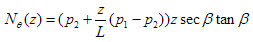
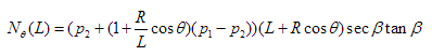
The above allow us to find the meridional and normal stresses at any point on the hopper given any two initial linearly-varying pressures p1 and p2, a length L from the virtual tip, and any height z above the virtual tip (even exceeding L). However, the position of most interest is the horizontal intersection (along the y-axis this time) between the hopper and the silo, where z = L. But that is not all. The sinusoidal variation of the radius with respect to the y-axis must be also included and thus z = L + Rcosθ, with θ = 0 at point A. Hence:
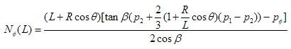
and
Other load cases top Δ
Further derivations will be made for the case of friction, where, for example, pf = μpn or for load patterns which do not follow a linear distribution. Taking friction into account, the above standard results for the meridional stress resultants (normal resultants remain unchanged) become respectively:
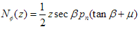
and
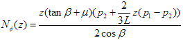
The equations are yet to be derived for any load patterns other than constant and linear.
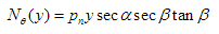
In all of the above cases, what is actually desired are the circumferential and meridional membrane stresses which are given by the following simple relationship:
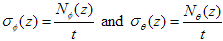
where t is the shell thickness.
Preliminary ABAQUS Modelling top Δ
Work has already begun on creating a functioning FEA model of a silo with the simplest case of a right-angled conical hopper. For this case, we aim to obtain a correlation between the FEA results and the membrane theory equations we derived, thus allowing us to use the ABAQUS model as a benchmark against which we may test other equations in the future for more complex elliptical geometries and eccentric axes.
The model will initially use an S4R element, meaning that it is a 4-noded, shell element with reduced integration (one integration point per element at its centre of gravity as opposed to a point per node in the S4 element; reduces calculation time for 3D geometries) and possible hourglass control to reduce mesh instability and potential for the hourglassing mesh phenomenon for reduced integration elements (ABAQUS, 2004).
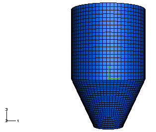
Fig. 13 - Preview of future EFA silo geometry and mesh for a conical right-angled hopper
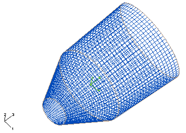
Fig. 14 - Closer look at the fine mesh of the future FEA silo model